Introduction
Recap_
This is a continuation of my previous post, Wolfram’s Wonderful World.
In the previous post I used a list zipper to implement a world with a focused element and defined all the 256 rules for Wolfram’s ECA. Additionally, the code can save a number of iterations for each rule to PNG files. The disadvantages of this
- the current implementation is a naive reinvention of the wheel
- no support for toroidal worlds
- list indexing with
!!isO(n)creates needless computational complexity - cell values could be computed in parallel
- all code is in one module called
Main
I’ll also bear in mind that running the code to generate the 256 2K images from the previous post took 79 minutes and 11 seconds.
I intend to resolve the first three issues with the code in this post, and hopefully developing a better data structure would allow me to easily implement a two-dimensional experiment, such as Conway’s Game of Life.
Related work_
The first work on comonadic computation of elementary cellular automata I found is from Dan Piponi. He also used a list zipper, like I did in the previous post, and then wrapped it into an instance of Comonad. Given the post is 15 years old (mad, right?), I thought I’d look around for any new developments. I stumbled upon Philip Zucker’s post which also shows a very similar list-zipper solution, and also makes reference to another implementation that doesn’t use a zipper, but simply a list which becomes longer with every evaluation.
There’s clearly a pattern here, which came naturally to me as well as it did to all the other developers approaching this problem. But unlike them, I had no idea what a comonad really is. Uhm, another type-systems magic box with some magic powers?
Another problem was that all these implementations are just toy examples with even more disadvantages than my implementation from the previous post: no parallelisation, no optimisation, no exports to image, no randomness. So I turned to /r/Haskell, where I stumbled upon a comment in which Edward Kmett linked to his own post from 2013. Compared to the others, this is quite advanced (as well as acomplished). His comonad solution uses memoization, implements generic Wolfram rules, and a way to display images in the browser. But the trouble is, if you’re a rookie like me, you won’t understand half of it! And on top of that I had troubles running it (dreaded Diagram).
But it shouldn’t be like this. The beautiful way in which this problem can be solved in Haskell should really be known to more programmers and scientists all around the world. If something as incomprehensible as the concept of __self in Python is still very much comprehended, then why wouldn’t the structure capable of implementing repeated computation become second nature?
Thanks to my expertcomrade haskeller friend Jules, I will aim to contribute my part to this great goal of converting the whole scientific comunity to Haskell (and the whole planet to vegetarians, innit?).
Let’s begin!
Comonads
The maths
I’ll start with a few observations what type of functions the type W uses:
fmap :: (a -> a) -> W a -> W a
extract :: W a -> a
double :: W a -> W (W a)
evolve :: (W a -> a) -> W a -> W a
The world W a is an instance of the Functor typeclass. Practically, it implements an fmap function that given a computational context holding some values it takes the values out of the context, transforms them, and returns them again wrapped inside the context. That’s also what happens when a function is mapped over a list: each list element is transformed but what is returned is still a list of the updated elements. Plot twist: lists are Functors.
On top of fmap, the world defines extract, double and evolve, which all look kind of fundamental. extract and double are inverses with respect to worlds: composing them yields an identity function over worlds.
:t extract . double
W a -> W a
:t fmap extract . double
W a -> W a
For comparison, here’s a Monad.
:i Monad
class Applicative m => Monad (m :: * -> *) where
(>>=) :: m a -> (a -> m b) -> m b
(>>) :: m a -> m b -> m b
return :: a -> m a
fail :: String -> m a
So, a monad is also a context, but on top of allowing functions to be mapped over the elements inside the context, it also supports a few more operations that allow us to work directly with contexts without having to always take the elements out, modify them, and put them back again:
- wrapping an element into a context with a function called
return(which is like the reverse ofextract!) - applying a function that takes an element and returns something wrapped in a context to elements inside a context without getting a double context back: that’s bind
>>=, and allows monadic computations to be chained one after the other in an almost “imperative” fashion! This is a bit like ourevolve, but the function is the other way around and>>=takes the context first and then the function, whileevolvetakes the rule first and then the world.
It seems to be related to what I wrote for W a, but something doesn’t click. So I asked comrade Jules.
The most common formulation of monads in category theory is not the standard one used in Haskell, although they are equivalent, the one used in Haskell is better adapted for use in computation. The formulation in category theory, for a monad m, has two operators:
return :: a -> m a
join   :: m (m a) -> m a
and has to be a functor, so has the operator:
fmap :: (a -> b) -> m a -> m bfrom this, you can define bind:
v >>= f = join (fmap f v)A co-monad, w, is then defined by flipping the direction of the arrows in these functions, so they have the following operators (while also being functors):
extract   :: w a -> w
duplicate :: w a -> w (w a)
It should then be obvious that, in the same way as return and join are “opposites”
extract . return = id
duplicate . join = id
This is a great explanation so I have included it here as it is. Thank you comrade! I now know that join is the inverse of double and extract is the inverse of return. How beautiful. This is what in category theory is called a dual, so a comonad is the dual of a monad.
The code
Now that I kinda know what it is, I had a look at the definition of a Comonad (imported from Control.Comonad):
:i Comonad
class Functor w => Comonad (w :: * -> *) where
extract :: w a -> a
duplicate :: w a -> w (w a)
extend :: (w a -> b) -> w a -> w b
Well would you look at that. extract is the same as my extract, duplicate is the same as my double, and extend is evolve! Tell me I’m not brilliant.
So I dumped those definitions and made W an instance of Comonad instead
instance Comonad W where
    extract (W _ x _) = x
    duplicate w = W (tail $ iterate left w) w (tail $ iterate right w)
    extend rule w = fmap rule $ duplicate w
Array of light
Better indexing
The code in the previous post indexes lists in O(n) in order to create the image. If the dimensions of the image are h and w getPixel gets called O(h * w) times. Moreover, since !! is O(n), then getPixel itself is O(n * w). This means imgRun is O(h^2 * w^2). Horrible!
getPixel must be O(1). This is when the disadvantage of the zipper kicks in. It was copacetic to not have an index and think all left and right dance moves on my infinite Lineland, but now I must to come back from the clouds and use Arrays (which, in Haskell too like in C, can be indexed in O(1)).
So, if I turn the list of generations in imgRun into an array, the operation itself will be O(h * w). But then each call of getPixel can use ! instead of !! which is O(1), thus causing getPixel to be O(1) too. Then imgRun becomes O(2 * h * w). Much better.
getPixel x y = showPixel $ image ! y ! x
image = fmap (listArray (0, n-1)) $ listArray (0, d * 2) generations
generations = run (wolframRule r) w n d
I used listArray from Data.Array, which takes a tuple of the array boundaries and a list and returns an array.
Arrays in Haskell
As I dreamed about the day when this project is complete and thought of multi-dimensional simulations, it occurred to me that maybe being able to use indexes isn’t that bad after all. In two dimensions or more neighbour computations become more funky and indexes are useful. Also, converting from lists to arrays at the last minute like above seems unnatural. So let’s try arrays then!
Haskellers on various forums seem pretty keen on telling people not to use arrays. The most troubles seem to occur when arrays have to change a lot, since behind the scenes there is a lot of memory being used. Thankfully, since I am interested in every step of the simulation, I don’t need mutable arrays, because I create a new one for each step. Array indexing is O(1), so if I implemented extract and extend over arrays they would also be O(1), same as in the zipper-list.
So I had a deeper look at Data::Array and it’s a bit uncanny. Arrays are something quite imperative, so thinking about using them in a purely functional language filled me with that strange mix of curiosity and fear that draws children to haunted forests in fairytales. And haunted it is…
:i Array
type role Array nominal representational
data Array i e
  = GHC.Arr.Array !i !i {-# UNPACK #-}Int (GHC.Prim.Array# e)
  	-- Defined in ‘GHC.Arr’
Which basically degobledygooks into something along these lines:
data Array i e = Array (i,i) [(i,e)]Array is actually a data structure formed of the following:
- a tuple (pair) of index-like values (which in Haskell are part of the typeclass
Ix), which delimit the lower and upper bounds of the array (signified by the typeiin the array definition above) - a list of tuples in which each index is paired with each array element (and values are signified by type
e)
Yet, the Array constructor is not exported by the module. I imagine that’s what it looks like, but turns out you can only use the array function to create an array.
As a computer engineer I have stumbled many times upon the 0-vs-1 debate about where arrays should begin. Ancient giants such as Cobol, APL, Fortran, Smalltalk as well as mathematical linguas like Matlab and Wolfram/Mathematica go for 1. Which makes sense… I guess? C-like and this century’s languages go for 0. But wait a minute, in Haskell you can have arrays start whenever the hell you want. So take an array that keeps the letters ‘m’, ‘a’, ‘d’ on indexes from 100 to 102:
a :: Array Int Char
a = array (100,102) [(100,'m'),(101,'a'),(102,'d')]
Arrays are a little bit rigid, for example one can’t pattern match over them[*] to get the bounds and the elements. The Data.Array includes a bunch of useful functions to compensate for that:
boundsreturns the tuple of bounds given the arrayelemsreturns the array elements given the arrayrangereturns a list with all the indexes in the array given the bounds
[*] (unless the BangPatterns language extension is used, which allows pattern matching with indexes)
λ> bounds a
(100,102)
λ> elems a
"mad"
λ> range $ bounds a
[100,101,102]
λ> a ! 101
'a'
So far, it looks like it does the job, but I can’t shake off this dirty imperative feel. I didn’t choose to write Haskell to see crap like this:
λ> a ! 1
*** Exception: Ix{Integer}.index: Index (1) out of range ((100,102))
Alas, this better be worth it!
Comonadic arrays
So here are Haskell Arrays, but they aren’t comonads. I want to use arrays but also the idea of an element being in focus, because it makes computation so easy and parallelisable. The focused element was embedded in W a because it was the element in the middle of two lists. In the case of arrays, the data type could be parametrised by an index, which fullfills the same role to represent the element in focus:
data W i e = W i (Array i e) deriving (Functor, Show)

instance Ix i => Comonad (W i) where
    extract (W i a)   = a ! i
    duplicate (W i a) = W i $ listArray (bounds a) (flip W a <$> (range $ bounds a))
    extend f w        = map f $ duplicate w
extract :: W i e -> e and extend :: W i e -> (W i e -> e) -> W i e look as expected.
How I got to duplicate :: W i e -> W i (W i e) : it should create a new world whose array is an array of worlds iterating through the range of indexes. range $ bounds a does this iteration. The data constructor for W takes the index first otherwise it can’t be parametrised in the comonad. Because of that, I need to flip the arguments of the data constructor, so W takes the world first and index last, so the constructor W a can be iterated over all indexes i in range $ bounds a with the same array a. The iteration is done with app <*> which is basically like an fmap and that’s all I’m going to say.
And that’s it. Those five lines of code basically implement the whole world.
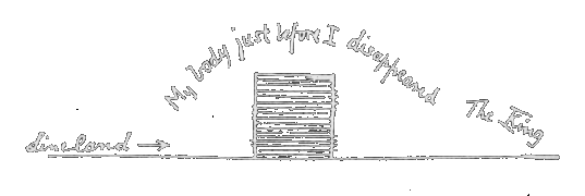
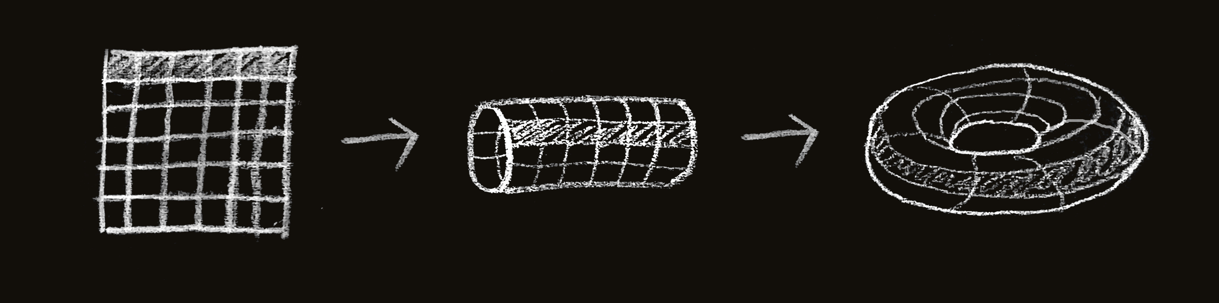
The world is your torus
Unlike lists, Arrays are finite. So if I created evolution rules that take a cell’s neighbours, the first and last cell would only have one. Instead, the first element can be the last’s element right neighbour and the last element could be the first element’s neighbour. This turns our linear world into something more like a ring. If the same thing is done over 2 dimensions, then the topmost elements will have the elements on the bottom line as neighbours and so on, which would make the world look like a torus.
For simplicity I chose to implement the left and right functions similarly to what I had with the zipper, so the actual indexing is done under the hood, and in the case a rule needs to be written left and right would handle the logic:
left, right :: (Ix i, Num i) => W i a -> W i a
left  (W i a)
    | i == 0    = W (snd . bounds $ a) a
    | otherwise = W (i-1) a
right (W i a)
    | i == (snd . bounds $ a) = W 0     a
    | otherwise               = W (i+1) a
The code (again)
Having implemented left and right above the code for the Wolfram rules can stay exactly the same. The wolframWorld has changed, since it needs to create an array and not a list. I also added a little helper arr function that gets the array out of the world structure and a run function to iterate through generations. Here is the code in its full glory:
{-# LANGUAGE DeriveFunctor #-}
module Main where

import Codec.Picture
import Control.Comonad
import Data.Array
import Data.Bits
import Data.Bits.Bitwise (fromListBE)
import Data.Word

--- Data Type
data W i a = W i (Array i a) deriving (Functor, Show)

instance Ix i => Comonad (W i) where
    extract (W i a)   = a ! i
    duplicate (W i a) = W i $ listArray (bounds a) (flip W a <$> (range $ bounds a))
    extend f v        = fmap f $ duplicate v

left, right :: (Ix i, Num i) => W i a -> W i a
left  (W i a)
    | i == 0    = W (snd . bounds $ a) a
    | otherwise = W (i-1) a
right (W i a)
    | i == (snd . bounds $ a) = W 0     a
    | otherwise               = W (i+1) a

arr :: Ix i => W i a -> Array i a
arr (W _ a) = a

run :: Ix i => (W i a -> a) -> W i a -> Int -> [W i a]
run rule w n = take n $ iterate (extend rule) w

-- Wolfram rules
wolframWorld :: Int -> W Int Bool
wolframWorld d = W d $ listArray (0, 2*d)
    $ (take d $ repeat False) ++ [True] ++ (take d $ repeat False)

wolframRule :: Word8 -> W Int Bool -> Bool
wolframRule x w = testBit x $ fromListBE (fmap extract [left w, w, right w])

wolframRun :: Word8 -> Int -> Int -> IO ()
wolframRun r n d = mapM_ putStrLn generations
    where
        generations = stringShow $ run (wolframRule r) (wolframWorld d) n

-- Show as string
stringShow :: [W Int Bool] -> [String]
stringShow ws = map (concat . map showCell . list) ws
    where
        showCell True  = "██"
        showCell False = "  "
        list (W i a) = elems a

-- Show as image
imageShow :: [W Int Bool] -> Int -> Int -> DynamicImage
imageShow ws h w = ImageRGB8 $ generateImage getPixel h w
    where
        getPixel x y = showPixel $ pixelArray ! x ! y
        pixelArray = listArray (0, h-1) $ map arr ws
        showPixel True  = PixelRGB8 0x00 0x00 0x00
        showPixel False = PixelRGB8 0xff 0xff 0xff

main :: IO()
main = sequence_ $ map save [0..255]
    where
        save r = savePngImage (imgPath r) (img r)
        imgPath r = "img/rule" ++ show r ++ ".png"
        img r = imageShow (run (wolframRule r) (wolframWorld d) n) n (2*d+1)
        n = 1024
        d = 1024
This magical bit of code does in 11 minutes what the previous bit of code did in 79 minutes. This is two and a half seconds to generate a 2K PNG. Not bad?
Introducing Flatland
2D array
It’s time to move on from the one-dimensional Lineland to a new and exciting two-dimensional world!
The best part of Haskell arrays is that the index doesn’t have to be a number. It could also be a tuple. This means I can use a pair (i,j) to parametrise the comonad, and a ! (i,j) to get the element at position (i,j) in the array, instead of creating an array of arrays, which is pretty neat!
There’s no change required to the data type and Comonad instance. The main difference between Flatland and Lineland is that a cell has eight neighbours instead of just two. So left and right must be replaced with functions that change the focus element into one of the 8 possible “cardinal points”. I have represented those with an enum, Move, and added a function neighbour which takes a cardinal point and a world and returns the new world with the new focus element. (Note: the World has been renamed to U)
data Move = N | NE | E | SE | S | SW | W | NW deriving (Bounded, Enum, Eq, Show)

neighbour :: (Integral i, Ix i) => U (i, i) a -> Move -> U (i, i) a
neighbour u@(U (i, j) a) move = case move of
    N  -> U (i,               (j + 1) `mod` w) a
    NE -> U ((i + 1) `mod` h, (j + 1) `mod` w) a
    E  -> U ((i + 1) `mod` h,  j)              a
    SE -> U ((i + 1) `mod` h, (j - 1) `mod` w) a
    S  -> U (i,               (j - 1) `mod` w) a
    SW -> U ((i - 1) `mod` h, (j - 1) `mod` w) a
    W  -> U ((i - 1) `mod` h,  j)              a
    NW -> U ((i - 1) `mod` h, (j + 1) `mod` w) a
    where
        h = height u + 1
        w = width  u + 1
The usage of mod implements the torus. Take a 6x6 grid. The cells on the 6th row will have a southern neighbour on the 1st row. The cells on the 6th column will have a western neighbour on the 1st column, and so on. Graphically, the transformation looks like this:
The functions height and width get the dimensions of the grid in order to calculate the modulus. The dimensions are encoded in the array’s bounds, which look like this: ((0, 0), (h-1, w-1)).
height, width :: (Integral i, Ix i) => U (i, i) a -> i
height (U _ a) = fst . snd . bounds $ a
width  (U _ a) = snd . snd . bounds $ a
Conway’s Game of Life
Since it deserves a post of its own, I’ll only use Conway’s Game of Life (aka Life) as a quick example. Life supports two states, Alive and Dead (True and False?) and only defines a single transformation rule. The transformation rule is as follows (thanks Wikipedia)
- Any live cell with fewer than two live neighbours dies, as if by underpopulation.
- Any live cell with two or three live neighbours lives on to the next generation.
- Any live cell with more than three live neighbours dies, as if by overpopulation.
- Any dead cell with exactly three live neighbours becomes a live cell, as if by reproduction.
The first step is a way to count the neighbours:
numNeighbours :: U (Int, Int) Bool -> Int
numNeighbours u = length $ filter id $ fmap extract $ map (neighbour u) [N ..]
With the occasion I found out about a little bit of Haskell syntactic sugar
- since
Nis the first element,[N ..]iterates through all the elements in theMoveenum filter iduses the identity function to check is the cell isTrueorFalse. The identity function simply returns the cell value, andfilteronly selects the values for which the functionidisTrue, thus it can be used to count the alive cells
Then the transformation rule codes into:
gameOfLife :: U (Int, Int) Bool -> Bool
gameOfLife w
    |      extract w  && (numNeighbours w < 2)          = False
    |      extract w  && (numNeighbours w `elem` [2,3]) = True
    |      extract w  && (numNeighbours w > 3)          = False
    | not (extract w) && (numNeighbours w == 3)         = True
    | otherwise                                         = extract w
The magic of Life is all about the initial configurations. There are a few famous ones, of which spaceships and pulsars and so on; I’ll try a glider, since it’s the simplest one, using only five alive cells.
To represent an initial configuration it is enough to list the cells which are alive and combine them using the incremental array update operator // with an array of False elements.
glider :: U (Int, Int) Bool
glider =  U (0, 0) xs
  where
    ys = listArray ((0, 0), (20, 20)) $ repeat False
    xs = ys // [ ((1, 3), True)
               , ((2, 2), True)
               , ((0, 1), True)
               , ((1, 1), True)
               , ((2, 1), True) ]
Final code
For now I’ll only implement a print to terminal and clear it between generations to display it like an animation. This can be done with rawSystem "clear" [] from System.Process. The full code is below. You can import it into an interactive shell and write runConway glider. Pressing any key shows the next generation.
{-# LANGUAGE DeriveFunctor #-}
module Main where

import Control.Comonad
import Data.Array
import System.Process (rawSystem)

--- Data Type
data U i a = U i (Array i a) deriving (Functor, Show)

instance Ix i => Comonad (U i) where
    extract (U i a)   = a ! i
    duplicate (U i a) = U i $ listArray (bounds a) (flip U a <$> (range $ bounds a))
    extend f u        = fmap f $ duplicate u

--- 2D world
data Move = N | NE | E | SE | S | SW | W | NW deriving (Bounded, Enum, Eq, Show)

height, width :: (Integral i, Ix i) => U (i, i) a -> i
height (U _ a) = fst . snd . bounds $ a
width  (U _ a) = snd . snd . bounds $ a

neighbour :: (Integral i, Ix i) => U (i, i) a -> Move -> U (i, i) a
neighbour u@(U (i, j) a) move = case move of
    N  -> U (i,               (j + 1) `mod` w) a
    NE -> U ((i + 1) `mod` h, (j + 1) `mod` w) a
    E  -> U ((i + 1) `mod` h,  j)              a
    SE -> U ((i + 1) `mod` h, (j - 1) `mod` w) a
    S  -> U (i,               (j - 1) `mod` w) a
    SW -> U ((i - 1) `mod` h, (j - 1) `mod` w) a
    W  -> U ((i - 1) `mod` h,  j)              a
    NW -> U ((i - 1) `mod` h, (j + 1) `mod` w) a
    where
        h = height u + 1
        w = width  u + 1

--- Game of Life
numNeighbours :: U (Int, Int) Bool -> Int
numNeighbours u = length $ filter id $ fmap extract $ map (neighbour u) [N ..]

gameOfLife :: U (Int, Int) Bool -> Bool
gameOfLife w
    |      extract w  && (numNeighbours w < 2)          = False
    |      extract w  && (numNeighbours w `elem` [2,3]) = True
    |      extract w  && (numNeighbours w > 3)          = False
    | not (extract w) && (numNeighbours w == 3)         = True
    | otherwise                                         = extract w

glider :: U (Int, Int) Bool
glider =  U (0, 0) xs
  where
    ys = listArray ((0, 0), (20,20)) $ repeat False
    xs = ys // [ ((1, 3), True)
               , ((2, 2), True)
               , ((0, 1), True)
               , ((1, 1), True)
               , ((2, 1), True) ]

--- Show as string
stringShow :: U (Int, Int) Bool -> [String]
stringShow u@(U (i, j) a) = map showRow $ [ U (k, j) a | k <- [0 .. height u] ]
    where
        showCell True  = "██"
        showCell False = "  "
        showRow (U (i, j) a)
            = concatMap showCell [ extract $ U (i, k) a | k <- [0 .. width u] ]

runConway u = do
    getLine
    rawSystem "clear" []
    mapM_ putStrLn $ stringShow u
    runConway (extend gameOfLife u)
Future work
The correct way to represent this into an image would be to create a GIF. I’ll do all that in the next post, together with exploring more configurations. Moreover, I’ll switch to parallel arrays because I can.
Bibliography
- Edwin Abbott, Flatland: A romance in many dimensions, 1884
- Dan Piponi, Sigfpe Blog, Evaluating Cellular Automata is Comonadic, December 2006
- Philip Zucker, Cellular Automata in Haskell, September 2017
- Edward Kmett, School of Haskell, Cellular Automata, November 2014
Haskell packages: