Motivation
Simulation gone rogue_
The other day I was reminiscing about simulations with my friends M. and J., and as such I remembered about one time in university when I let a lousy simulation of Conway’s Game of Life run basically indefinitely on a lab machine. Tragically, it was shut off by the lab administrator after it’s been running for two months, and for reasons not worth mentioning I was never able to recover the results.
In fairness, I didn’t even care at the time - our assignment has been to run a thousand iterations, and out of curiosity I had set it to run for much more than that and forgotten about it. Then M. mentioned how if run for long enough, Game of Life manifests into self-similar patterns. The same claim I had also seen in recent reading (and to be fair, it seems intuitive enough - have you ever looked at the thing?). The whole conversation gave me this uncontrollable thirst and urge to run it again - this time, in better conditions, with better code - if only to see some pretty fractalicious pictures worth printing on t-shirts, hanging on walls, tattooing on butts when drunk, whichever is your fancy.
With the help of another friend, professor at Uni of Bath, I managed to get my hands onto an entire book on the subject. Moreover, as I dived into some studies about complexity science, I was happy to see a bunch of their models (say, the forest fire, and the sandpile) can also be expressed as cellular automata. My plan is thus to implement a generic framework to run such models, and this series of posts should document my journey through the complex realms of the meaning of life.
In the rest of this post I’ll be introducing the problem and solve the elementary automata in naive Haskell, as well as quickly present a form of graphical output.
Haskell is a harsh mistress_
Disclaimer: I’ve been really looking forward to write something in Haskell, as I haven’t really written it since the compiler. Because of that, I must re-teach myself a lot of things, and shake off the imperative/procedural dust that has settled over me in the past few years. I find the best way to write better Haskell is to start with the naive solution and slowly increment into something more compact, more efficient, and of course, ever more beautiful - so I’ll do that.
One last thing. This post is dedicated to my friend Zeme, a true Haskell monk and a lover of beauty, who pointed me at modules and functions I would’ve never known otherwise.
Cellular automata
Cellular automata (CA) is the name given to range of discrete models studied over a bunch of disciplines, including but not limited to maths, computing, physics, theoretical biology and complexity science. At the core, a CA is simply a system of very basic, identical agents, that are somehow distributed in space, and follow some rules of evolution over discrete time steps. In most cases they interact with each-other based on their topology, that is, the state of one cell is only influenced by the state of neighbouring cells.
CAs are also called tesselation structures. The reason for this is because cells may be other shape than square. Covering a surface with more complex shaped cells whilst also maintaining the homogeneity of the grid has become an art of its own. But for now, let’s fall back to square lattices.
CA were first discovered and discussed by Stanislaw Ulam in the 40s for the purpose of studying crystal growth at the Los Alamos lab. At about the same time his colleague, the polymath John von Neumann, researching automation and self-replication, was able to apply the same idea and create, or discover, the first artificial system capable of replicating itself. This evolved into the von Neumann automata, of which more later.
Interestingly enough, one-dimensional or elementary automata came much later, with Stephen Wolfram’s paper in 1983, describing a system of rules and classifications for celular automata in only one dimension. Wolfram was fascinated by the idea that rules so simple can generate so complex and unpredictable a behaviour, lurking with fractals, randomness, and even Turing-completeness. Wolfram dedicated a thousand pages to these systems. I humbly dedicate them this article.
Elementary CA
Take an infinite toroidal band representing our one-dimensional world, which I shall call Lineland.
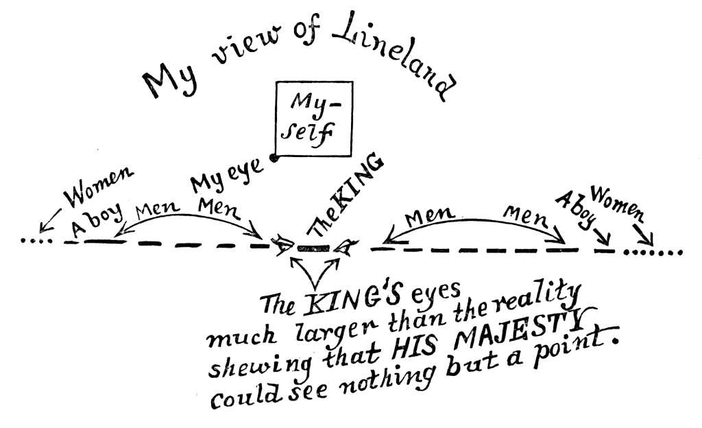
This world is populated by point-sized cells, represented by 1. The empty space between them is represented by 0. At each generation, the value of the current cell is decided by the value of the neighbours in the previous generation. So for generation G, cell N, and convolution f:
valG(N) = f(valG-1(N-1), valG-1(N), valG-1(N+1))
Wolfram devised a very compact system of generating all possible CA rules for this configuration, called Wolfram codes. Given that all convolutions are applied to three-cell tuples, and each cell has two possible values, then there are 223=28=256 possible convolution rules to be generated. The three neighbour tuples are all 23 possible combinations of three bits so can be represented the numbers from 0 to 7. Conveniently, the binary expansion of the rule number has also 8 bits, so a direct mapping can be made.
For example, 30 has the following binary expansion (in Little Endian convention):
[0, 1, 1, 1, 1, 0, 0, 0]
Thus, Rule 30 is expressed as a truth table as:
000	001	010	011	100	101	110	111
0	1	1	1	1	0	0	0
The same truth table as for the following logical function:
valG(N) = valG-1(N-1) XOR (valG-1(N) OR valG-1(N+1))
Sometimes, for example for rule 90 (which is simply the XOR of the neighbours), the logical function provides a lot of insight into why the CA ends up looking the way it does. But more on that in the following episodes!
Implementation
Wolfram Rules
Sounds very basic - all one needs is to map from the rule number, which is an integer in the range [0..255], to its binary expansion expressed as a list of bits. The first thing that comes to mind for implementing the above would be a list comprehension.
In Python, that would look something like this (respecting Little Endian-ness):
def wolframRule(x):
	return [(x / pow(2, i)) % 2 for i in range(8)]
The equivalent list comprehension in Haskell:
wolframRule :: Int -> [Int]
wolframRule x = [(x `div` 2^i) `mod` 2 | i <- [0..7]]
Recall that Haskell is strictly typed, and that for soundness I should only support rules for the range [0..255], which is equivalent to an 8-bit integer. The type Word8 in Data.Word is exactly that. Moving on to the output type: why create a list of integers when I need 1 bit to represent each of the results? An ideal type signature for the rule function would be, instead, something like: Word8 -> [Bool].
For this, having a look at Data.Bits, I found the function testBit, with the following signature:
:t testBit
testBit :: Bits a => a -> Int -> Bool
Given a (potentially infinite) array of bits and an integer n, testBit returns the value of the nth least significant bit as a boolean. Word8 is both a number and an 8-bit-long instance of type Bits, so getting each of the 8 bits in turn with testBit produces a list of Bools that is the binary expansion.
wolframRule :: Word8 -> [Bool]
wolframRule x = [ testBit x i | i <- [0..7]]
Now I’ll get serious, turn the list comprehension into a map, and get rid of that nasty magic number - the code should be able to know what’s the bit size of a Word8 input without me telling it it’s 8 bits; that’s what finiteBitSize does:
wolframRule :: Word8 -> [Bool]
wolframRule x = map (testBit x) [0..finiteBitSize x-1]
Now that we have a way to generate all the rules, before we can apply them, let’s start looking at the data structure representing the world.
Life in Lineland
The intuitive way to represent our world, Lineland, would be with an infinite list. But since we need to calculate the value of a unique cell, it would be nice we had the ability to “focus” on a specific element in this list. This is basically the concept of a zipper in Haskell, which is defined as an idiom that uses the idea of “context” to the means of manipulating locations in a data structure.
The nice thing about a zipper is that it allows a coder to implement iterative structures without thinking of an iterator, or without even trying to order or count the elements at all. Moreover, more than focusing on a cell, we also want to be able to shift left and right to calculate its neighbours, so we can be rid of that nasty N index we were previously working with and work directly with the cells and their neighbours.
cG = f(left(c)G-1, cG-1, right(c)G-1)
To express that in Haskell (no Python example this time, since this stuff can’t really be expressed in Python, because Python simply isn’t cool enough), let’s define a data structure where a central cell of generic type a is surrounded by two lists of cells of type a. This data structure also allows navigating to the left and right of the focused cell.
data W a = W [a] a [a]

left, right :: W a -> W a
left  (W (l:ls) x    rs ) = W    ls  l (x:rs)
right (W    ls  x (r:rs)) = W (x:ls) r rs
Now I want to be able to map functions over all the cells inside the world, since it’s really just a list, but I can’t do that directly, since the list is wrapped into this W. This is easily solved by making W an instance of Functor and defining fmap.
instance Functor W where
fmap f (W as x bs) = W (fmap f as) (f x) (fmap f bs)
extract :: W a -> a
extract (W _ x _ ) = x
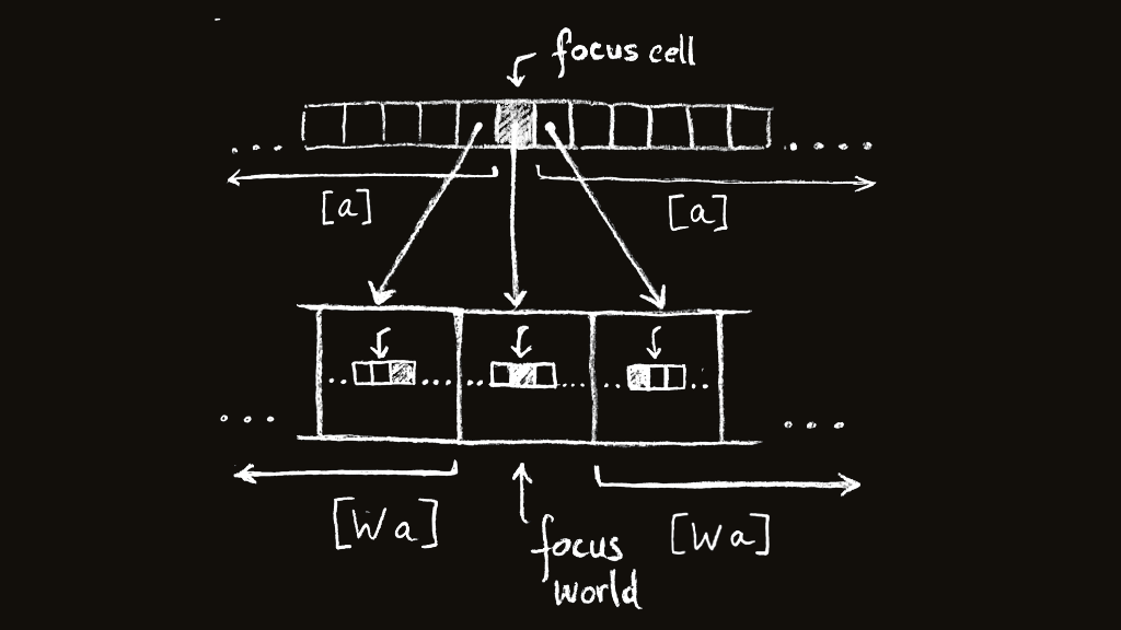
double :: W a -> W (W a)
double w = W (tail $ iterate left w) w (tail $ iterate right w)The transformation rules will be applied repeatedly over the world W a, and the updated world should be returned as a result. To do that, we need to look-behind at the previous generation, which is also a world, extract the cells’ values, calculate the convolutions, and wrap them back into a world. This is what the extract and double functions are for. extract only gets the “focused” cell out of a world, while double creates a world of worlds, where the original world becomes the focused element, and each of the left and right leftovers are made of lists of worlds for each cell from the original world to be in focus. It makes sense after a while, trust me. This drawing helps:
To match the above, the rules themselves must take a world and return a cell - the same type signature as extract: rule :: W a -> a.
Now, because rules extract a cell from a world, and we apply the rule over a world of worlds, after one iteration we will be left over with a plain world again, which allows us to iterate infinitely over the structure for as many generations as we want, since the iteration has the same type for its domain and codomain.
evolve :: (W a -> a) -> W a -> W a
evolve rule w = fmap rule $ double w

evolveN :: (W a -> a) -> W a -> Int -> [ W a ]
evolveN rule w n = take n $ iterate (evolve rule) w
Rules again
Since all cells in Wolfram’s worlds can be either alive or dead, then we can use a Bool to represent their values. This will make our world of type W Bool. We can also think of the rules in terms of both logical and binary operations.
For example, recall Rule 30:
valG(N) = valG-1(N-1) XOR (valG-1(N) OR valG-1(N+1))
If we were to hard code it onto our world, then it would look something like this:
rule30 :: W Bool -> Bool
rule30 w = lc /= (cc || rc)
    where lc = extract $ left  w
          rc = extract $ right w
          cc = extract w
Now to generalise: let’s take a quick look at our wolframRule
wolframRule :: Word8 -> [Bool]
wolframRule x = map (testBit x) [0..(finiteBitSize x-1)]
Conceptually, we want something that takes a rule number x (of type Word8) and a world and returns a cell, that is, after applying wolframRule to it. That means we’ll apply testBit x over the specific number between 0 and 7 that is represented in binary by the three values of the current cell and its neighbours. So if the current cell is dead, i.e. 0, and the neighbouring cells are both alive i.e. 1, then testBit x 5 will be the value of the current cell in the next iteration, since 5 is 101 in binary. Intuitively, that would look like this:
wolframRule :: Word8 -> W Bool -> Bool
wolframRule x w = testBit x $ cellsToNum w
    where
        cellsToNum w = lc + 2 * cc + 4 * rc
        lc = fromEnum $ extract $ left  w
        rc = fromEnum $ extract $ right w
        cc = fromEnum $ extract w
Ugh. Verbose. Ugly. A lot of repetition. Uneccessary stuff to convert the binary representations to integers just because they’re lists of Booleans. Not to mention the sum should be written as a fold. My mate Z. pointed me at Data.Bits.Bitwise, where I found fromListBE :: [Bool] -> Int which does exactly what our binary expansion sum combined with fromEnum do.
wolframRule x w = testBit x $ fromListBE (map extract [left w])
The meaning of forever
Now suppose we create some world w, and try to create 100 generations of Rule 30, it’s simply just evolveN (wolframRule 30) w 100.
Whatever you do, don’t try to run this code yet! Or try, and remain paralysed by the meaning of forever (until you run out of memory unless of course you Ctrl-C and it stops abusively printing 0s on your screen). Recall I mentioned infinite lists.

Haskell, like the Paralysed Horse, may have grasped the meaning of forever, but us mortals have to constrain ourselves to finite lists. So I truncated the world by taking d elements from the left side, the focused element, and d elements from the right side.
Note that (for now) we have no toroidal property. One should watch out and only appy left and right before truncating the infinite lists, otherwise the first element in the list won’t have a left neighbour and vice-versa. This is not how one should write Haskell, but alas, I want to see some pretty pictures already!
To make printing easy, I wrote a function that maps extract over a world and flattens it to a list. The finished simulation ends up being a simple list of lists.
truncateD :: Int -> W a -> W a
truncateD d (W ls x rs) = W (take d ls) x (take d rs)

list :: W a -> [a]
list (W ls x rs) = reverse ls ++ [x] ++ rs

run :: (W a -> a) -> W a -> Int -> Int -> [[a]]
run rule w n d = map (list . (truncateD d)) $ evolveN rule w n
First run
I have no idea how to make images in Haskell, and right now I just want to see what it does. Bet you do too. Add a quick printing function and a default world with one alive cell in focus to start with, and we’re up and running. Here’s the final code:
module Main where

import Data.Bits
import Data.Bits.Bitwise (fromListBE)
import Data.Word

--- Data Type
data W a = W [a] a [a]

instance Functor W where
    fmap f (W as x bs) = W (fmap f as) (f x) (fmap f bs)

extract :: W a -> a
extract (W _ x _ ) = x

double :: W a -> W (W a)
double w = W (tail $ iterate left w) w (tail $ iterate right w)

left, right :: W a -> W a
left  (W (l:ls) x    rs ) = W    ls  l (x:rs)
right (W    ls  x (r:rs)) = W (x:ls) r rs

--- Run a simulation
evolve :: (W a -> a) -> W a -> W a
evolve rule w = fmap rule $ double w

evolveN :: (W a -> a) -> W a -> Int -> [ W a ]
evolveN rule w n = take n $ iterate (evolve rule) w

run :: (W a -> a) -> W a -> Int -> Int -> [[a]]
run rule w n d = map (list . (truncateD d)) $ evolveN rule w n
    where
        list (W ls x rs) = reverse ls ++ [x] ++ rs
        truncateD d (W ls x rs) = W (take d ls) x (take d rs)

--- Generic Wolfram Rules
wolframWorld :: W Bool
wolframWorld = W (repeat False) True (repeat False)

wolframRule :: Word8 -> W Bool -> Bool
wolframRule x w = testBit x $ fromListBE (fmap extract [left w, w, right w])

--- Print to terminal
showCell :: Bool -> String
showCell True  = "██"
showCell False = "  "

printRun :: Word8 -> W Bool -> Int -> Int -> IO ()
printRun r w n d = mapM_ putStrLn generations
    where
        generations = map showGen $ run (wolframRule r) w n d
        showGen cs = concat $ map showCell cs
Try printRun 30 wolframWorld 100 100.
Don’t forget to install the bitwise package if you don’t have it. If you’ve never run Haskell before, read this.
Here’s mine (had to zoom out of my terminal a lot):
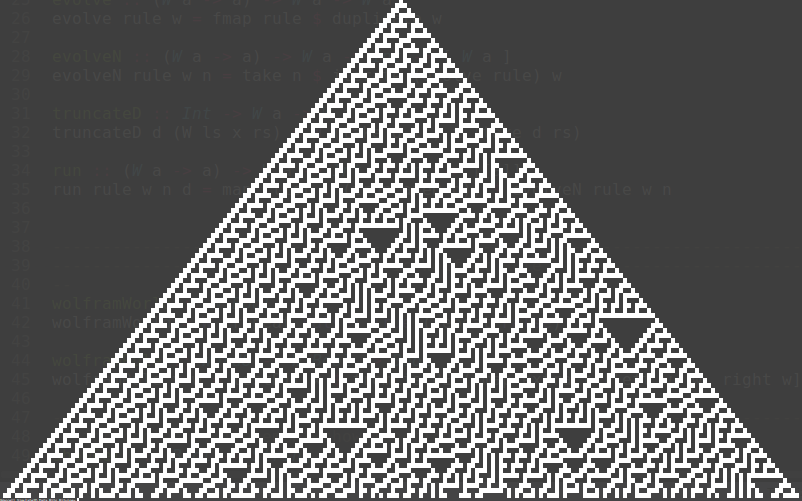
Huh? you’re not impressed? Fine. Then have a look at the mathematics again. No? Have a look at the code again. It’s basically 30 lines excluding comments and imports, and it’s not even the best Haskell can be. Still not impressed? Then have a look at this shell, Conus Textile. Just. Look at it. This is called beauty. Inhale and say it, after me: beauuutiful.

Exporting to image
I’m always lost when it comes to libraries. I just can’t stand the process of choosing and maintaining them. So I started by asking around what’s a good library to export images in Haskell, and decided to pick the one that works out of the box, no questions asked. Below are the names that are most thrown about:
Attempt 1: diagrams
- Pros: Looks like a fantastic package for vector graphics, beginner-friendly, with intuitive data types
- Cons: it’s notoriously slow and I can’t manage to install the right one (there’s significant type changes between versions and that’s just a hassle!)
Attempt 2: gloss
- Pros: uses openGL, handles vector graphics
- Cons: wait… it shows pictures on the screen? what is this, MATLAB?
Attempt 3: JuicyPixels
- Pros: you give it a pixel mapping and dimensions and it saves an image
- Cons: I don’t care, it works
Introducing JuicyPixels: exports nice data types called Image and Pixel. Juicy. You can create a pixel by assigning it integer RBG values, and generate images with the generateImage function:
:t generateImage
generateImage :: Pixel a
  => (Int -> Int -> a)  -- pixel value function for pixel (x,y)
  -> Int                -- Width in pixels
  -> Int                -- Height in pixels
  -> Image a
x and y can be the list indexes for our list of lists simulation and we can use a function to return an alive cell black and a dead cell white (i.e. getPixel x y). We can also use hex colour names, because Haskell knows these are numbers. 0xff and 0x00. Juicy.
And finally, let’s add a main function that iterates through all the Wolfram rules and generates images for a given dimension, starting with a world with only one living cell in the middle. To combine multiple IO() results into one we use sequence_.
showPixel :: Bool -> PixelRGB8
showPixel True  = PixelRGB8 0x00 0x00 0x00
showPixel False = PixelRGB8 0xff 0xff 0xff

imgRun :: Word8 -> W Bool -> Int -> Int -> DynamicImage
imgRun r w n d = ImageRGB8 $ generateImage getPixel (d * 2+1) n
    where
        getPixel x y = showPixel $ generations !! y !! x
        generations  = run (wolframRule r) w n d

main :: IO()
main = sequence_ $ map save [0..255]
    where
        save r = savePngImage (imgPath r) (imgRun r wolframWorld n d)
        imgPath r = "img/rule" ++ show r ++ ".png"
        rs = [0..255]
        n  = 1024
        d  = 1024
Don’t forget to import the Codec modules and install the juicypixels package to get them.
import Codec.Picture
import Codec.Picture.Types
Results
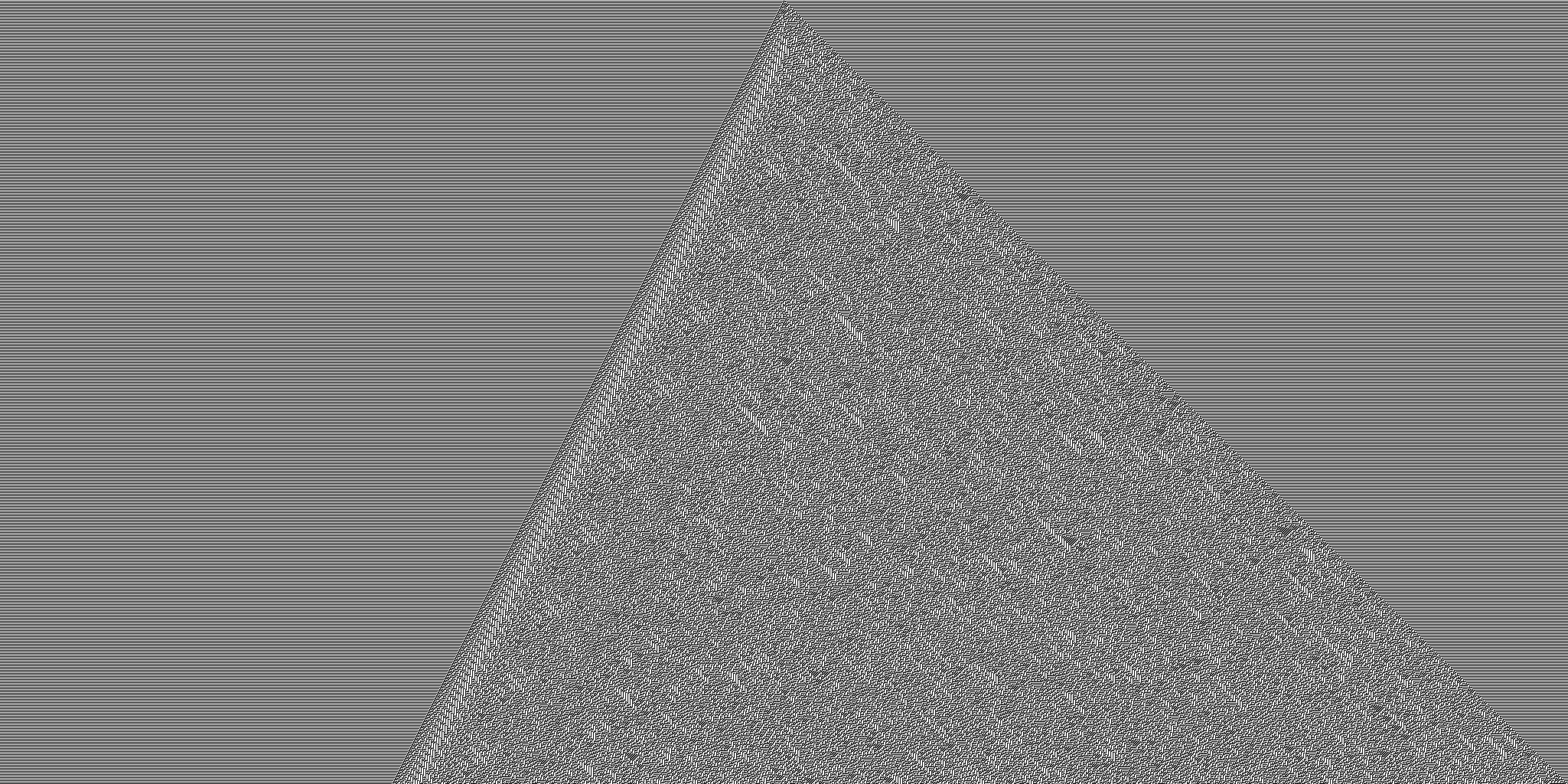
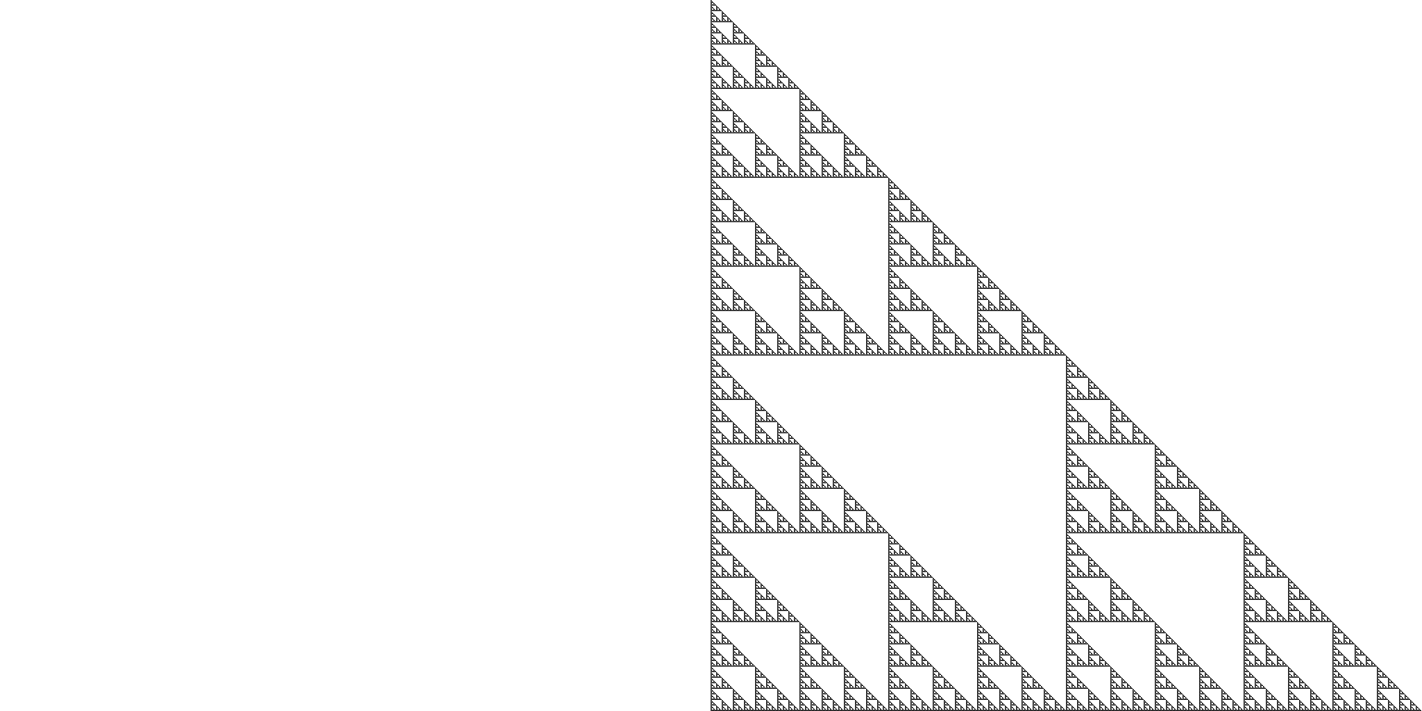
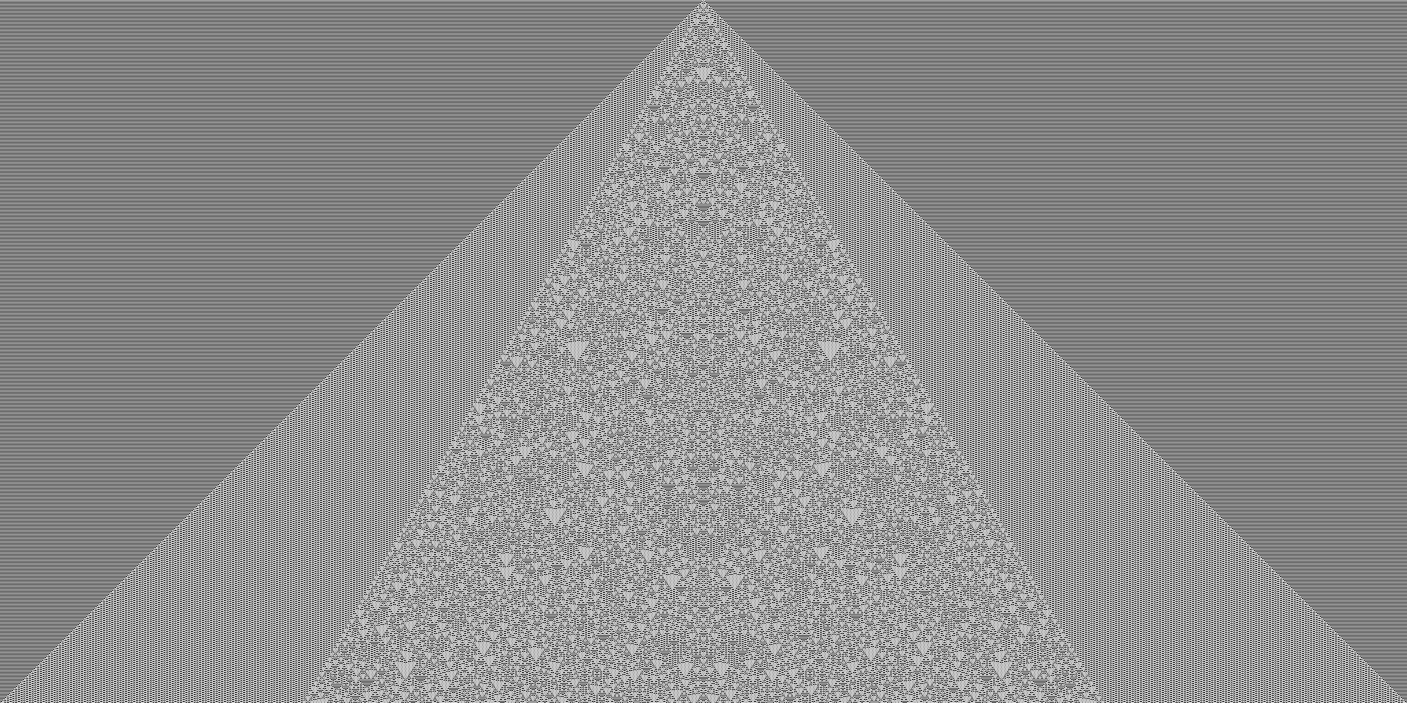
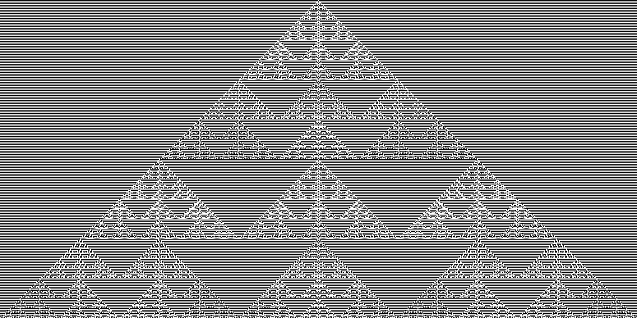
I generated 256 2049x1024px images, and it took around an hour to export them all. That’s quite slow, and I’ll briefly touch upon why in the self-critcism section below. Most of the images coming out were very simple, but some others were clearly self-similar and fractalicious (Sierpinski triangles bonanza!) and very complex. Some of them were honestly freaking uncanny. Like rule 45. Here are my favourites:
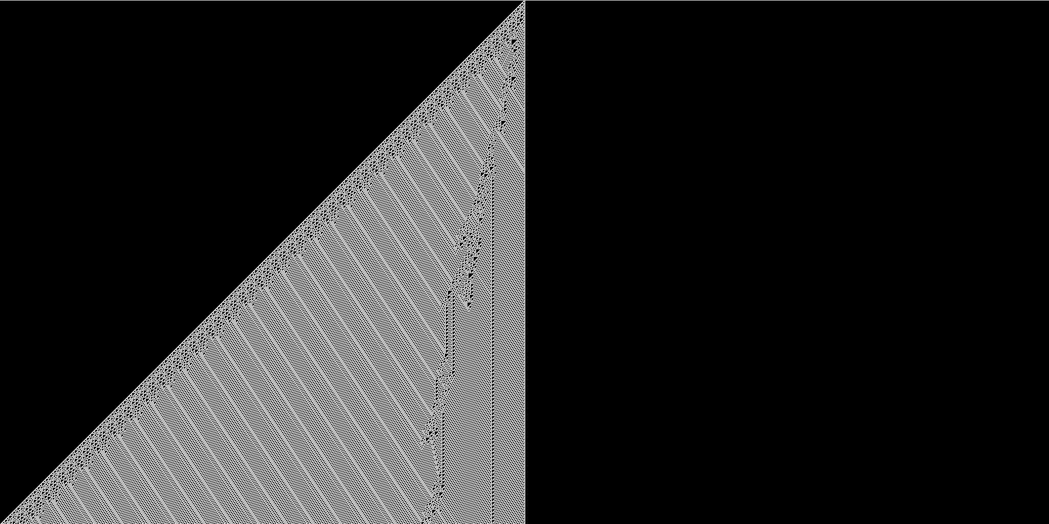
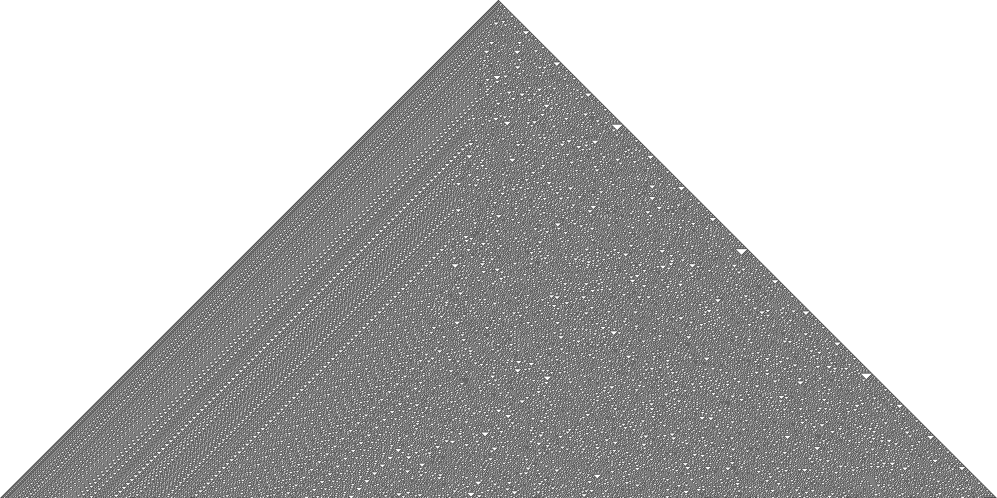 Rule 30
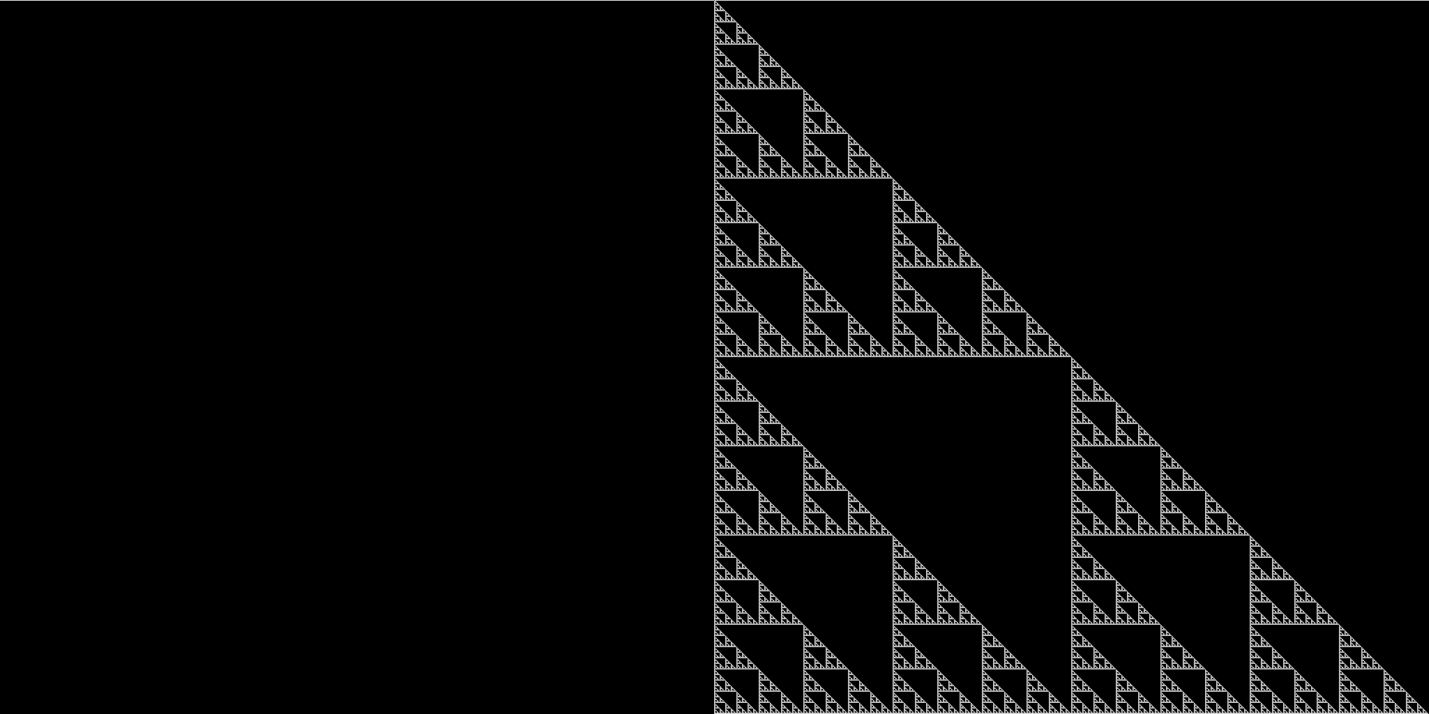
 Rule 45
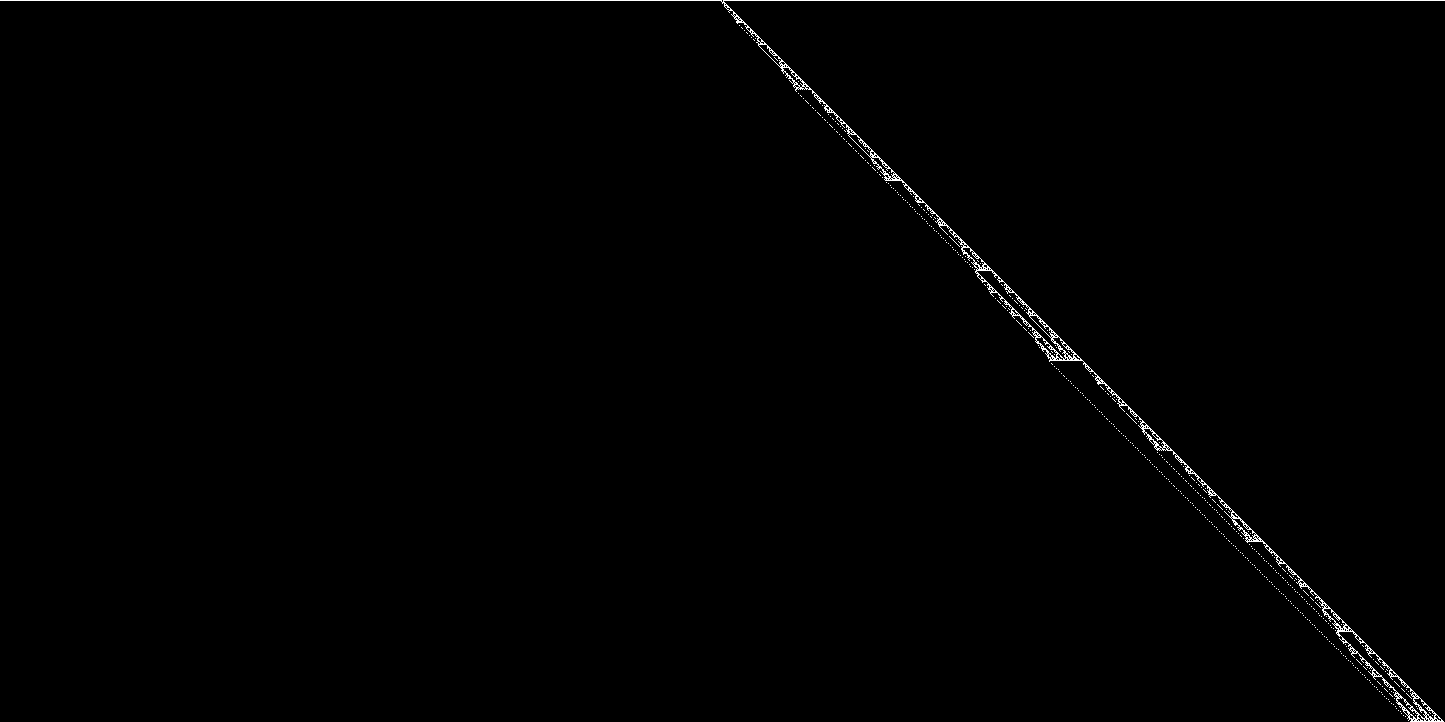
 Rule 57
 Rule 60
 Rule 73
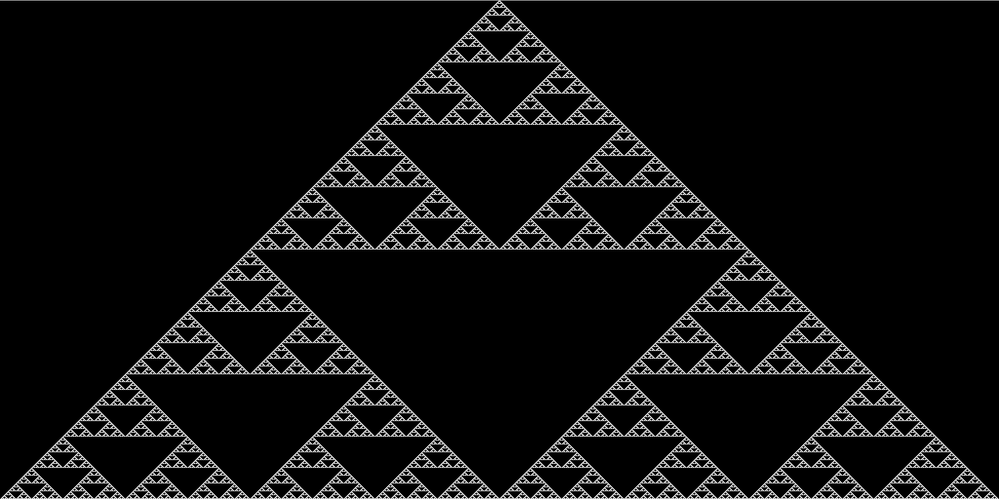
 Rule 90
 Rule 105
 Rule 137
 Rule 150
 Rule 161
 Rule 195
 Rule 225
Future work
The goal of this post has been achieved, namely to simulate elementary CA in Haskell and generate images. But the code could be better, and the pictures could be prettier. I will address the shortcomings of the code in future parts of this article, as well as prepare it to be extended from Lineland to Flatland.
Self-criticism
The code compromises efficiency for readability, which is expected of many naive Haskell implementations. On top of that, the truncation function simplifies an important feature or problem of cellular automata, namely computing cell values at the edges - we have assumed the world is infinite and trimmed bits of it, ignoring the case in which the world is toroidal: the first cell actually influences the evolution of the last, since they are neighbours. This can be easily implemented into the left and right functions when considering finite worlds. The goals for the next post are thus:
- support toroidal worlds
- use instances of Haskell’s data types for
W a, as the current implementation is a naive reinvention of the wheel - parallel computation of cell values in the next generation
- less computationally expensive image generation (list indexing with
!!isO(n), unlike a C-array where it’sO(1)) - split code into modules
Improvements
A number of improvements could be made to observe more interesting phenomena. Probabilistic evolution and random initial configurations came to mind after seeing Mandelbrot’s random Koch curve. The Random monad promises a lot of adventures:
- randomly generate initial worlds
- randomly assign colours
- probabilistic rules
Annex: Your first Haskell simulation
I’d be honoured if this were the first time you ever considered writing Haskell. To make it much smoother for you to join the dark side (we have cookies too) here’s a couple of instructions for getting up and running.
If linux or mac, simply install haskell-platform with your package manager. On windows, get the Haskell Platform from here. It will install the package manager cabal, the Glasgow Haskell Compiler GHC, and for windows also an interactive command line interface, WinGHCi.
Make sure you have the right packages installed. Pop a terminal/command line window open and get the bitwise and juicypixels packages with cabal install bitwise juicypixels.
Open a file, dump the code in it, save it as Hascell.hs or whatever, and then run
ghc -o Simulate Hascell.hs
This command compiles it into a binary that you can run, Simulate.
Otherwise, if you like to play with it interactively, run ghci Hascell.hs in your terminal / WinGHCi.
References
- Edwin Abbott, Flatland: A romance in many dimensions
- Stephen Wolfram, Statistical mechanics of cellular automata, Rev. Mod. Phys. 55, 601 – Published 1 July 1983
- Stephen Wolfram, A new kind of science, Wolfram Media, 2002.
- Learn You a Haskell for Great Good, Functors, Applicative Functors and Monoids
- Learn You a Haskell for Great Good, Zippers
- StackBuilders, Image processing with Juicy Pixels and Repa
Packages